An introduction to spatial data in R

Published 1 Oct 2021 7 min read code

Project

NB: This was originally a tutorial given to Space Lunch members on 6th October 2021. This is an adapted version. The original version, which uses a marine example, can be found on the Project page.

Introduction

This is going to be an introduction to a simple workflow for spatial data in R using rasters. I will assume you have some basic knowledge about spatial analyses and co-ordinate systems. This is not meant to be a documentation of the full suite of spatial analysis available in R. Some simple ways of plotting data is covered.

Rasters are stored spatial data in a gridded format.

Each grid cell contains a single value. E.g. temperature, elevation, species richness
Often stored in three dimensions (e.g. latitude, longitude and time).
The main R package for handling rasters is raster.

We will consider a common workflow of associating rasters with spatial point data (e.g. lat and long). I will be sticking to base R throughout.

Introducing rasters

Loading from file

Rasters can be acquired from a range of sources, such as government agencies. There are also R packages to interface directly with online databases but for another time. Often they are saved as an nc file (network Common Data Form) that is imported as a raster with layers and assigned a spatial projection. You’ll see below that other dependent packages are loaded with raster but you won’t need to load each one manually.

You can load a raster from a local nc file using the function raster::brick. The :: denotes calling a function from a specific package without loading it with library. Good for quick and dirty functions you won’t use frequently, bad if you are using the package multiple times.

my_raster <- brick("raster_data.nc")

I will cheat and use the built in function in raster to query WorldClim for mean annual temperature.

library(raster)

## Loading required package: sp

temp <- getData("worldclim",var="bio",res=10)

## Warning in getData("worldclim", var = "bio", res = 10): getData will be removed in a future version of raster
## . Please use the geodata package instead

Subsetting rasters

Subset rasters by layers using basic square bracket subsetting for lists.

temp <- temp[[1]] # Subset only the first layer - mean annual temperature

Here I have selected mean annual temperature since we do not need the other variables.

Plot rasters

We can use the basic plot function to view the raster data.

plot(temp)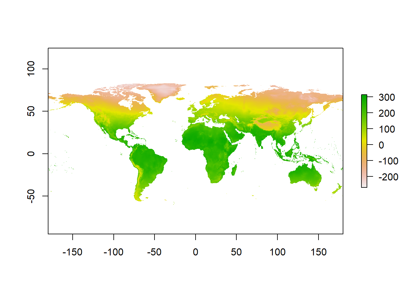

Figure 1: Average annual temperature

The default colour scale is horrendous so we will change it to the viridis scale. Here’s an example of using ::. I don’t need the entire viridis package. This is to make a continuous colour palette of 20 colours. And add a title to the graph.

plot(temp, main = "Mean annual temperature", col = viridis::viridis(n = 20))

Figure 2: That’s better

There’s one last issue to deal with before this data is ready. WorldClim stores temperature data multiplied by 10 for space saving so we need to divide by 10.

Manipulating rasters

Rasters can be manipulated by base functions. E.g. addition or subtraction between rasters or layers. There are many other functions for analysing rasters and doing spatial analysis (e.g. interpolation) but we won’t cover that here.

temp <- temp/10
plot(temp, main = "Mean annual temperature", col = viridis::viridis(n = 20))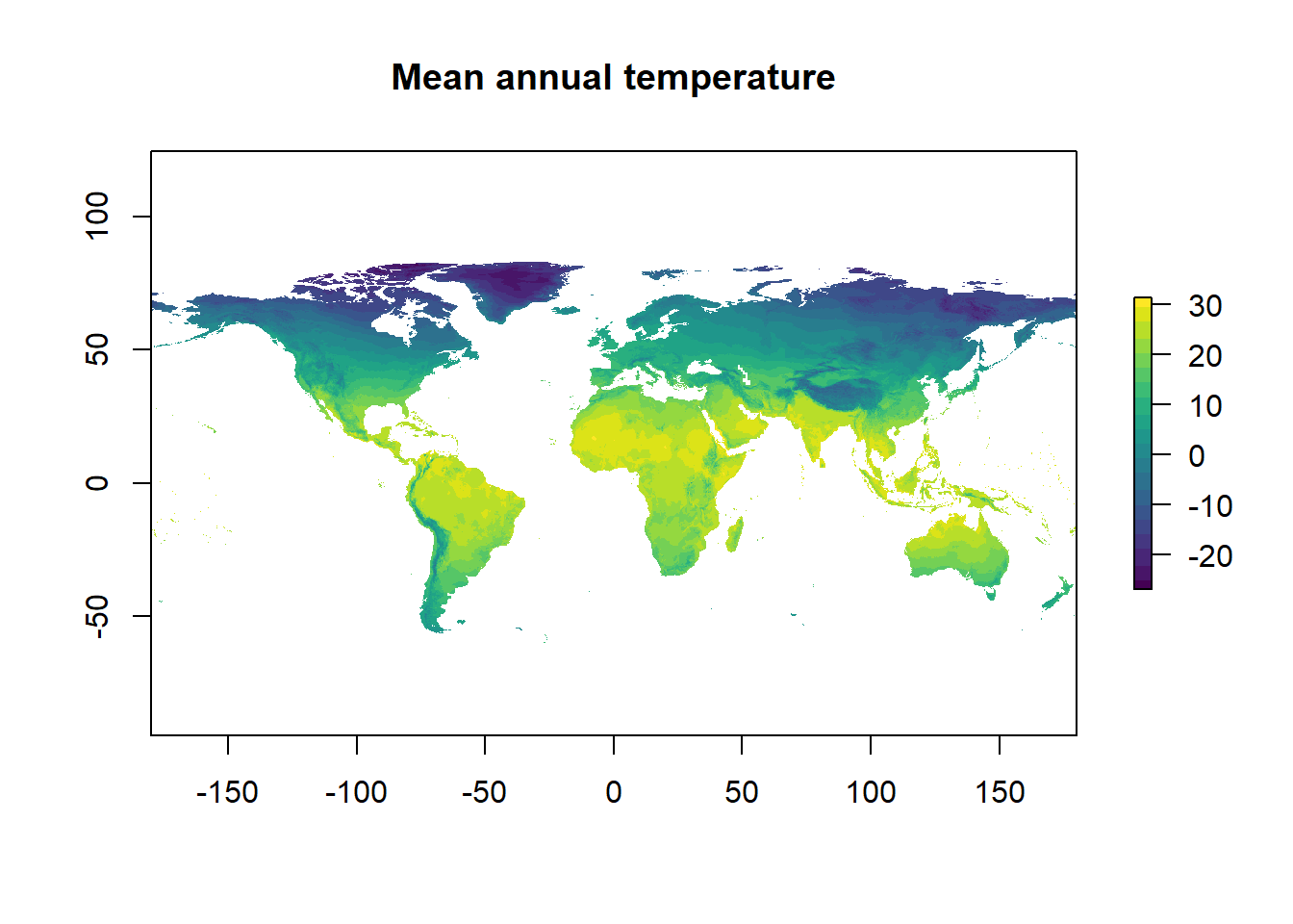

Figure 3: That’s much much better

Spatial point data

I usually encounter spatial data in the form of decimal latitude and longitudes representing species occurrences or sampling sites. You may already have these data from your own work but for demonstration purposes I will show how to query an online database to get species distribution points from GBIF. This requires an Internet connection and the R package rgbif.

Let’s query GBIF occurrence points for an widespread bird: The house sparrow (Passer domesticus).

You need the unique identification key for the species you want. name_suggest can help with that so you don’t have to manually search GBIF.
The data comes as a list with some metadata. .$data is the actual occurrence records. The dot . is a placeholder meaning it represents an R variable (e.g. a dataframe). This is commonly used in tidyverse and piping via magrittr. It is also a cheat’s way of using base functions within a pipe.
Co-ordinates are stored as decimalLatitude and decimalLongitude. I’ve removed any missing values manually but occ_search has a variable called hasCoordinate to return records with lat/long data.
rgbif gets a max 500 records each time by default (limit). Use page to denote which record number to start at.

library(rgbif)
# get ID key for bird
bird_key <- name_suggest(q ="Passer domesticus", rank='species')$data$key[1]
# get occurrence points
bird_points <- occ_search(taxonKey = bird_key) # Get all records, max 500 (see variable limit)
# exclude metadata
bird_points <- bird_points$data
# remove NA latitude or longitude
bird_points <- bird_points[!is.na(bird_points$decimalLatitude),]

Since I’ve only searched for one species, the workflow is simple. If I wanted multiple species I would have to use lists and a function like sapply. See help file for occ_search for an example. Avoid for loops.

Plot spatial data

Let’s look at the global distribution of points. I will use the base maps package for a simple, low resolution and unprojected world map in R (not recommended for more professional output). The maps package can also be used in ggplot2 via borders(database = "world", fill = NA) or geom_polygon(data = map_data("world"), aes(x=long, y = lat, group = group), fill = NA, col= 1); coord_map() may help in these cases.

library(maps)
map("world") # get basic world map
title(main = "The distribution of house sparrow") # plot title
points(decimalLatitude ~ decimalLongitude, bird_points, pch = 16, col = 2) # plot points
legend(x = -150, y= -50, legend = "occurence", pch = 16, col = 2, bty = "n")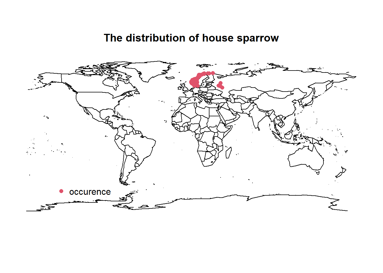

We see that the 500 points from GBIF come mainly from around northern Europe. Here is a good point to check for sampling bias of points or any potential erroneous points - I will ignore this step for this demonstration.

For more advanced mapping in R check out ggmaps, which can interface with Open Street Maps (free) and Google Maps (for a fee), and osmdata, which interfaces directly with OSM and allows you to customise which features to include - check out the related tutorial about mapping cities in R in the Space Club folder or online.

Putting it all together

Now we have all the data we need, let’s combine the datasets and plot the occurrence data with the temp raster.

plot(temp, main = "Mean annual temperature", col = viridis::viridis(n = 20)) # temp
points(decimalLatitude ~ decimalLongitude, bird_points, pch = 16, col = 1) # bird

Figure 4: The distribution of sparrows with mean annual temperature

Let’s do some simple extraction of data.

What range of temperatures do house sparrows live in?

We can use our new species distribution points to query the raster and extract values corresponding with the occurrence points. The function to query a raster is raster::extract. The same can be used within tidyverse::mutate.

# Get temp
temps <- extract(temp, SpatialPoints(cbind(bird_points$decimalLongitude, bird_points$decimalLatitude)), method = "bilinear")
# Add new column
bird_temps <- cbind(bird_points, temps) 
# Remove missing temps
bird_temps <- bird_temps[!is.na(bird_temps$temps),]

method = "bilinear" tells the function to interpolate the average of the nearest 4 cells around the spatial point. This is like a mini version of buffer which will interpolate values within a buffer around a point. If spatial accuracy is not paramount (like here where we have a global scale raster), then this method might reduce the chance of extracting a NA value. The default is to query the exact coordinate.

Our final dataset contains 500 observations.

Missing data at this stage could be from a mismatch between the accuracy of the spatial points and the resolution of the raster. Or plain errors in the spatial coordinates.

Now we can plot the distribution of temperatures:

hist(bird_temps$temps, main = "Temperature distribution of house sparrows")

We can see they live between -2.7 and 8.2 °C, which here reflects the fact that all the points were sampled from northern Europe.

Finally, we can plot the relationship between temperature and latitude:

plot(temps ~ decimalLatitude, bird_temps, pch = 16)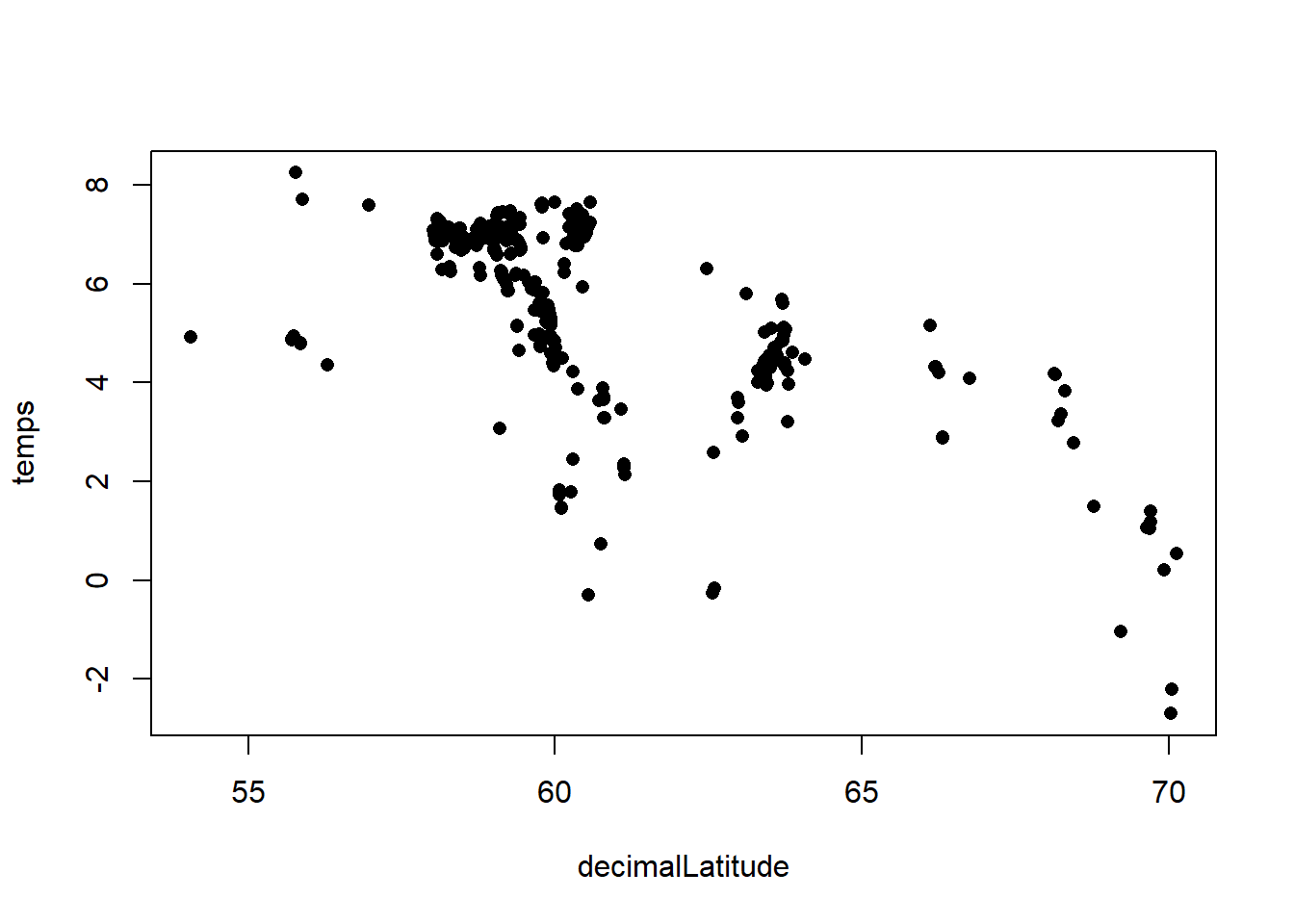

End

code R stats

Jacinta Kong

Postdoctoral Fellow

My research interests include species distributions, phenology & climate adaptation of ectotherms.