This tutorial was originally presented to NERD club on 4/2/2020.
City maps
Consider yourself a hipster?
Do the clean lines and natural materials of modern scandi make you feel at home?
Is your basic coffee order a flat white? ☕
If the answer to all the above is YES, then here’s a present for you!

But wait! This poster costs €30 (thereabouts) online!
See example.
That’s approximately 9 flat whites you could have had.
☕☕☕☕☕☕☕☕☕
Can you make this in R?, you ask, asking for a friend.
Fear not. You can make this yourself in R!
Maps in R
In this tutorial we will replicate a poster like this. We will need R and powerpoint to put in the final touches. You could do it fully in R but powerpoint will make our lives a bit easier. In summary, it requires a bit of GIS wrangling to code in what you want to display.
The data is freely available from Openstreetmap, for proprietary haters out there. I will refer to it as OSM.
We will be following this tutorial.
Setup
You will need to install the relevant packages: osmdata, tidyverse and sf.
#install.packages("osmdata", "tidyverse", "sf")
library(osmdata)
library(tidyverse)
As you can see this will use tidyverse and I will be using piping. Don’t worry if you are not a master at piping. The code is written.
In a nutshell, instead of function2(function1(X)) to apply function 1 then function 2 to X, you type x %>% function1() %>% function2(). I.E. take X, apply function 1, then apply function 2 to the resulting output. Overall it’s easier to read, hence it’s ‘tidy’.
OSM data
OSM stores various features you can explore under available_features(). You can see what is under each feature with available_tags("<insert feature name here>").
1. Get city co-ordinates
For this example we will make a map of Dublin. First we need the latitude and longitude of Dublin. If you want to modify the extent of your map, this is where you change the co-ordinates.
city_coords <- getbb("Dublin Ireland")
#city_coords <- c(-6.391,53.2644,-6.114883, 53.416) # to get all the M50
2. Get map features
Roads
We can get roads by querying OSM for the GPS co-ordinates for Dublin and saving it to a variable called roads.
roads <- city_coords %>% #pipe!
  opq() %>% # create query for OSM database
  add_osm_feature(key = "highway",
                  value = c("motorway", "primary",
                            "secondary", "tertiary")) %>%
  osmdata_sf() # save it as an simple features format
roads
Streets
We can do the same for streets.
streets <- city_coords%>%
  opq()%>%
  add_osm_feature(key = "highway",
                  value = c("residential", "living_street",
                            "unclassified",
                            "service", "footway")) %>%
  osmdata_sf()
Water
Can’t forget the Liffey and the canals. Sadly the ocean cannot be mapped.
water <- city_coords%>%
  opq()%>%
  add_osm_feature(key = "waterway", value = c("canal", "river")) %>%
  osmdata_sf()
3. Plotting
Time to call ggplot2 and plot our map.
map <- ggplot() +
# roads
geom_sf(data = roads$osm_lines,
inherit.aes = FALSE,
color = "grey", # colour of feature
size = 0.8, # Size on map
alpha = 0.8) + # transparency
# streets
geom_sf(data = streets$osm_lines,
inherit.aes = FALSE,
color = "#ffbe7f",
size = 0.2,
alpha = 0.6) +
# water
geom_sf(data = water$osm_lines,
inherit.aes = FALSE,
color = "steelblue",
size = 0.8,
alpha = 0.5) +
# extent to display
coord_sf(xlim = c(city_coords[1],city_coords[3]),
ylim = c(city_coords[2],city_coords[4]),
expand = FALSE) +
# remove axes
theme_void()
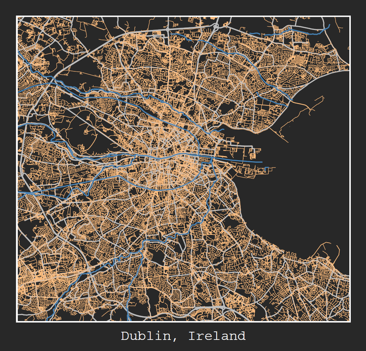
map4. Labels
At this point it is easier to save the file and add text in powerpoint but if you want to try your hand at ggplot’s annotation features go ahead.
Here I’ve done one in a dark colour scheme.
theme_colour <- "#282828" # dark theme

dark_map <- map +
  labs(caption = "Dublin, Ireland") +
  theme(axis.text = element_blank(),
        plot.margin=unit(c(1,1,1,1),"cm"),
        panel.grid.major = element_line(colour = theme_colour),
        panel.grid.minor = element_line(colour = theme_colour),
        plot.background = element_rect(fill = theme_colour),
        panel.background = element_rect(fill = theme_colour),
        plot.caption = element_text(size = 24, colour = "white", hjust = 0.5, vjust = -2, family = "mono"),
        panel.border = element_rect(colour = "white", fill=NA, size=2),
        axis.ticks = element_blank())

dark_map
Saving our map
ggsave(plot = dark_map, filename = "NERD/dark_dublin.pdf", width = 11, height = 8.5, device = "pdf", dpi = 300)If all of that was too much, there’s an R package for it. https://github.com/lina2497/Giftmap
There is also a website
Extra details
Less is more but if you really want to put more features:
Other water bodies
extra_water <- city_coords %>%
  opq()%>%
  add_osm_feature(key = "natural", value = c("water")) %>%
  osmdata_sf()

dark_map +
   geom_sf(data = extra_water$osm_polygons,
          inherit.aes = FALSE,
          fill = "steelblue",
          colour = NA,
          alpha = 0.5) +
  geom_sf(data = extra_water$osm_multipolygons,
          inherit.aes = FALSE,
          fill = "steelblue",
          colour = NA,
          alpha = 0.5) +
  # extent to display
  coord_sf(xlim = c(city_coords[1],city_coords[3]),
           ylim = c(city_coords[2],city_coords[4]),
           expand = FALSE)
Parks
Nature reserves including Dublin Bay
park <- city_coords%>%
  opq()%>%
  add_osm_feature(key = "leisure", value = c("park")) %>%
  osmdata_sf()

dark_map +
   geom_sf(data = park$osm_polygons,
          inherit.aes = FALSE,
          fill = "darkgreen",
          colour = NA,
          alpha = 0.3) +
  geom_sf(data = park$osm_multipolygons,
          inherit.aes = FALSE,
          fill = "darkgreen",
          colour = NA,
          alpha = 0.3) +
  # extent to display
  coord_sf(xlim = c(city_coords[1],city_coords[3]),
           ylim = c(city_coords[2],city_coords[4]),
           expand = FALSE)
End
That’s the gist of using OSM in R. You can use the same code to make any map, e.g. for a paper.
Jacinta Kong
Postdoctoral Fellow
My research interests include species distributions, phenology & climate adaptation of ectotherms.