Statistical modelling Part 1
Introduction
This is a static version of the learnr tutorials for the Statistical Modelling practicals.
Welcome! In two practicals and in three lectures we will be looking at statistical modelling.
We have progressed beyond the realm of doing stats by hand and basic statistical tests like t-tests are not appropriate for the types of data we will look at or the hypotheses we test. R will be the tool we will use.
In these sessions, we will focus on the practical aspects of applying statistics (implementation & interpretation) with real data – not on the theory or mathematical proofs – in fact, nearly all the relevant theory has been introduced to you in previous lectures.
The practicals and lectures will feed off each other and these will also build upon the previous lectures and practicals. All concepts in this practical are assessable and relevant to the lectures. I expect you to be up to date with the module material.
The demonstrators are available if you have questions about the concepts or have technical issues with running the practical. Please talk to them, they get lonely. They will be checking in and making sure you are keeping to time.
What is statistical modelling?
Recall from the lectures:
Statistical models are logical mathematical or statistical descriptions of what we believe to be important in a biological system.
We use models to:
- Make sense of a complex and messy real world and its data
- Formulate new theories
- Test our understanding of a biological system
- Formulate hypotheses
- Make predictions
- Make evidence-based decisions
- Run simulations – “what if…?”, what happens if we change something?
If our model doesn’t match what we observe from empirical data, that’s OK! We can refine our model (our hypothesis) to better match what we observe. That’s the Scientific Method.
Remember!
To paraphrase: all models are wrong but some can be useful
Types of models
Models can be characterised in several ways depending on what they describe:
- Theoretic models describe processes – explored here
- Empirical models describe data – explored in lectures and in the next practical
Some biological systems can be described both ways.
Models can be placed on a spectrum of simple to complex, and specific to general.
Models can also be described based on their precision, realism and generality. But these trade-off – No one model can perfectly capture all these qualities.
All types of models are based on assumptions or require information about the biological system. Models describe a biological system with some limitations.
The best model to use depends on the intended question.
Variables vs parameters
Distinguishing between variables and parameters is important in statistics, particularly for modelling.
Variables
These are quantities that change with each iteration of a statistical model. E.g. the predictor (independent) variable and the response (dependent) variable.
Parameters
These are quantities that do not change with each iteration of a statistical model. They are often a constant and often represent the assumptions about our biological system we make to model it. If we change the fundamental assumptions of the model, then the value of the parameter may change. Often the value of the parameter is unknown to us and need to be parametrised from empirical data.
A variable could switch to being a parameter or vice versa depending on the experimental design and hypothesis tested, which in turn determines the statistical model. These decisions should be made when planning an experiment, not during or afterwards.
We will go through the process of parametrising in the next practical and in the lectures.
Practical information
In these practicals we will look at a theoretic model of a predator-prey interaction.
The aim is to understand how statistical models can be applied to biological data.
The majority of this practical will focus on the practicalities of designing experiments and collecting data, which we covered earlier in the module.
I recommend taking your time with these practical and the concepts because they are fundamental to biological statistics you are likely to encounter again (plus are highly relevant to your final report). There is no need to rush.
Learning objectives
This practical is split into three parts with distinct learning objectives (recommended time to spend):
Part A: Building a theoretic model (20 mins)
- Know how a biological process can be described by a statistical model
- Understand how statistical models are applied to answer real world biological questions
Part B: Designing an experiment (20 mins)
- Apply your knowledge about experimental design and hypothesis formulation to a biological problem in practice
Don’t spend too long on Parts A and B, move through them and the CA quickly. Part C is the most important part and will take the most time.
Part C: Collecting data (2 hours)
This is the main activity of the practical.
- Know how to organise a spreadsheet and fill in a spreadsheet with data following the principles of tidy data
You will be uploading your data to Blackboard. In the next practical we will be analysing the aggregated & anonymised class data set and using that to answer CA questions.
Continuous Assessment
I recommend finishing the CA before Part C. The CA is worth 10% and is due at the end of the prac. There is a total of 10 marks.
The CA aims to assess your understanding of the concepts in this practical and your ability to apply the concepts in practice.Part A: Theoretic models
In the previous practical you looked at a killer T cell digesting a pathogen. This infection response is a biological process and is analogous to a predator (e.g. a lion) hunting a prey (e.g. zebra), or a robot (a “predator”) cleaning up an oil spill (its “prey”).
You started to compose a Scratch model. Although the Scratch model comprises of pictures and code blocks, under the hood these blocks represent computer code, and more abstractly a mathematical processes. Thus, the Scratch model is an implementation of a statistical model of a biological system – the infection response.
This model was simple – too simple to be realistic. The killer T cell captured any and all pathogens touching it whereas in reality, a killer T cell may only target a few pathogens at a time or sequentially. This is also true for animal predators who hunt. Most predators need time to catch and process their food before their next meal.
We can conceptualise a more realistic representation of an infection response, or more abstractly a predator-prey interaction. By breaking down what we observe to be important about the infection response into variables and assumptions, we can build our own theoretic model (describing a process) of an predator-prey interaction from scratch.
What is a predator-prey interaction?
In a predator-prey interaction we have two variables:
- Predator
- Prey
If we think about what we consider to be important in a predator-prey interaction, searching for and handing prey two mutually exclusive aspects. We can then make the following statements, or assumptions, about the predator-prey interaction:
- A predator randomly searches for prey
- A predator can only “search” a fixed area per unit time (search rate)
- A predator can only eat one prey at a time – it must “process” (i.e. digest) the prey before it can begin searching for the next one (handling time)
- Handling time and searching activity are mutually exclusive
- Prey randomly move around independently of the predator (e.g. it does not slow down or speed up when the prey is near)
- Both the predator and the prey move at the same speed and at a constant speed
- Both the predator and the prey only move within a fixed area (e.g. their habitat), they cannot leave.
- The numbers of predators and prey are fixed at the start of the experiment (i.e. they do not replicate while the model is running, prey numbers can only decrease, predator numbers stay the same)
- Each predator-prey interaction lasts a fixed amount of time (total time)
These same statements can be applied to an infection response or to any analogous scenario – merely replace “predator” and “prey” with the relevant terms.
Discussion
If you thought our model is too simplistic, you are probably right but in modelling philosophy some degree of simplification or abstraction is perfectly acceptable because models are only representations of reality, they are not meant to copy the real world right down to the minutiae.
Functional responses
Infection responses, predator-prey interactions… they can be generally classified as functional responses. Luckily for us, there are already well known analytical (mathematical) models of functional response that we can use.
There are multiple types of functional responses (labelled with Roman numerals: I — IV). Each of these models represents a different hypothesis about functional responses and mathematically describes a different relationship between our two variables (e.g. the killer T cell and the pathogen, or a predator and its prey). You can read more about functional responses by running vignette("functional_responses").
The assumptions we make above are based on a Type II functional response model, which is common in biology. You can read about the full derivation by running vignette("TypeII_models").
The Type II functional response model is a good example of a general model – it has been used to describe animal predators eating prey (e.g. Holling’s disc equations) or enzymes catalysing reactions (e.g. Michaelis-Menten equation). We can also use it to describe the immune response of the previous practical.
It doesn’t matter what the mathematical symbols represent biologically, maths is a universal language that describes the underlying biological process. Here, we are applying it to an general predator-prey scenario involving students and plastic counters.
A Type II functional response
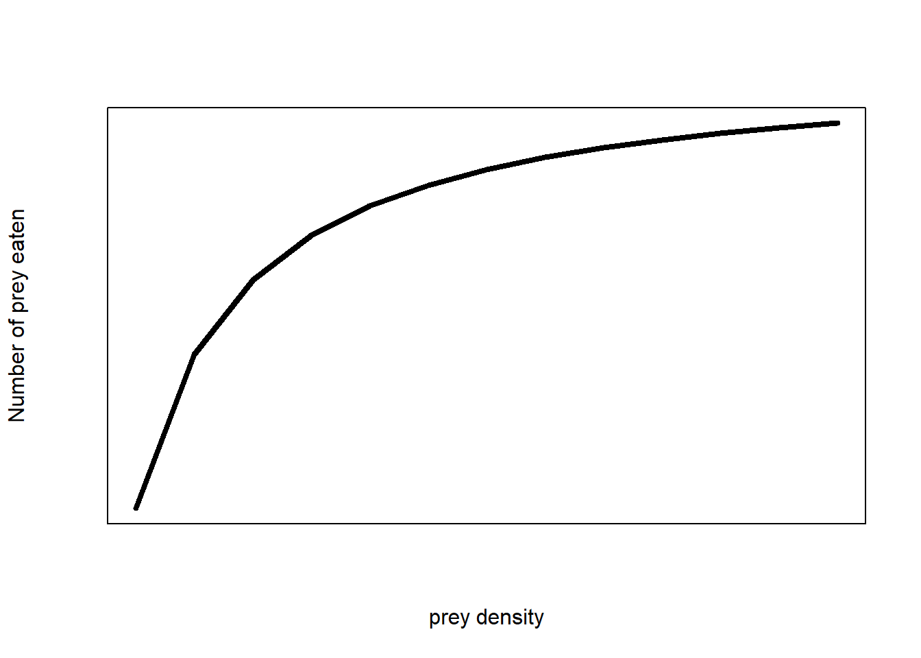
(#fig:funct_resp)Type II functional response of a predator-prey interaction
Discussion
Maybe something like:
“The number of prey eaten rapidly increases at low prey densities and gradually plateaus to a maximum number of prey eaten at higher prey densities.”
The mathematical model of the figure above is:
\[H_a=\ \frac{a\times H\times T_{total}}{1+a\times H\times T_h}\]
You should read the full derivation in the documentation file to see how we’ve turned our earlier assumptions into mathematical expressions – run vignette("TypeIImodels") in Console or via the Packages tab (click StatsModels -> User guides).
Let’s go through what the letters and numbers mean and how they link to our model assumptions.
- \(H\) is the number of prey within a fixed area (prey density, number per area). This is our predictor variable. We decide what values to use before our experiment
- \(a\) is the search rate or attack rate. It is the search area per unit time of a prey. This is a parameter that we do not know and that we calculate from our data.
- \(H_a\) is the number of prey captured. We record this at the end of our experiment as our response variable.
- \(T_{total}\) is the total time a predator spent hunting prey (time). This is a constant parameter that we decide before we start the experiment based on our assumptions.
- \(T_h\) is the time a predator spends digesting a single prey (time per prey). This is a parameter that we do not know and that we calculate from our data. In functional response models, this is called handling time.
You’ll see that we know the value of some of these parameters already and some we need to calculate from our data.
Discussion
Finding our unknown parameters
How do we estimate these unknown parameters from our data (e.g from the figure above)?
Actually, the hyperbolic nature of the Type II makes it challenging to extract this information – and certainly beyond the expectations of this module. But we can use mathemagics to turn this hyperbolic relationship into a straight line by a process called linearising. And straight lines are easier to manipulate or interpret – something we expect you to be able to do in this module.
The linearised Type II equation is:
\[\frac{1}{H_a}=\ \frac{1}{a}\times\frac{1}{H\times T_{total}}+\frac{T_h}{T_{total}}\]
The full derivation is accessible in vignette("TypeIImodels"), we won’t go though how this is derived here, but you do need to understand this equation:
- \(\frac{1}{H_a}\) is the inverse of our response variable – the number of prey eaten
- \(\frac{1}{a}\) is the inverse of our unknown search rate parameter
- \(\frac{1}{H \times T_{total}}\) is the inverse of our predictor variable (prey density) and the total predator-prey interaction time
- \(\frac{T_h}{T_{total}}\) is our unknown handling time divided by the total predator-prey interaction time
Discussion
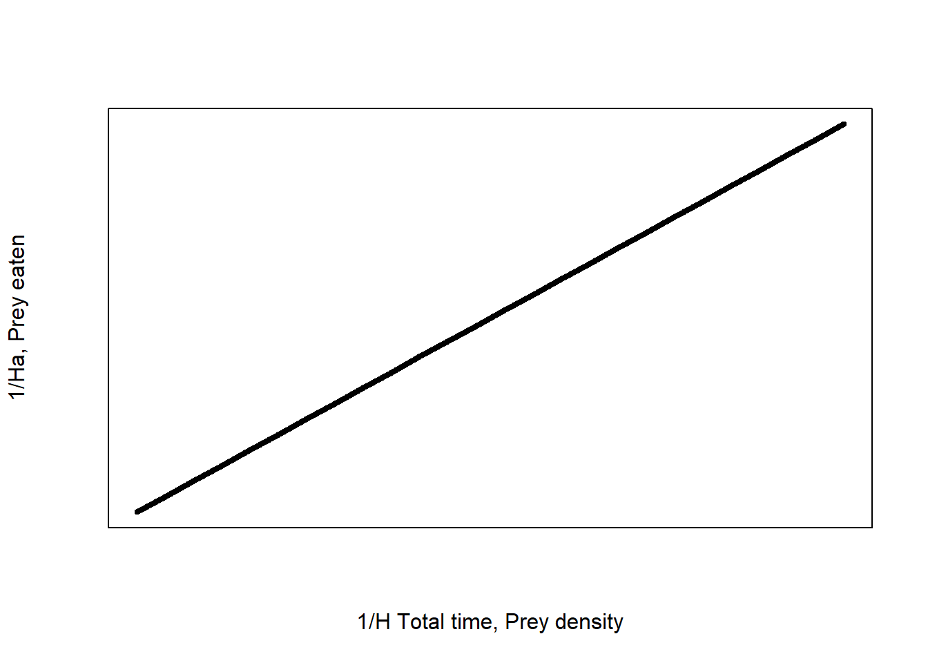
Figure 1: Linearised type II functional response of a predator-prey interaction
The linearised function has the general form \(y = \beta_1 x + \beta_0\) which is a straight line. \(y\) is the response variable, \(x\) is the predictor variable, \(\beta_1\) is the slope or gradient of the line, and \(\beta_0\) is the intercept of the line. We will see this notation again in the lectures.
This linear form allows us to estimate the coefficients for the linear equation where y = \(\frac{1}{H_a}\) and x = \(\frac{1}{H\times T_{total}}\).
From the linearised Type II equation we can see that:
\[Slope=\ \frac{1}{a}\]
\[Intercept=\ \frac{T_h}{T_{total}}\]
We can calculate the slope and intercept from regression and then do some algebra to find \(a\) and \(T_h\):
\[a=\frac{1}{slope}\]
and
\[T_h = T_{total} \times intercept\]
Now we have our model, we need to parameterise it and find the values of our unknown parameters.
For the rest of the practical we will look at the question:
Unlike the previous practical, we are going to investigate this question by conducting a real experiment but it is possible to build an equivalent simulation in Scratch.
That’s the end of Part A. Check in with your demonstrator. Take a break. Stand up. Shake your limbs. Breathe.
You’re doing great!
Part B: Designing an experiment
The predator-prey experiment
You have been provided some plastic counters, a stopwatch, a piece of paper and a jar with a lid. You are the predator and the counters are your prey. The piece of paper is your arena and the jar is for collecting prey that you have captured.
You will be working in pairs – one of you will be the predator, the other will be the observer (keeping track of the time, recording the data). You will need a computer between you for entering and uploading data.
The protocol is simple:
- Spread out the desired number of counters on the A4 sheet randomly. Do not move counters around once landed
- The predator will close their eyes and use their index finger to randomly tap around the arena at a constant search rate called out by the observer. The observer has a stop-watch and tells the predator when to tap.
- If the predator touches a counter, they need pick it up and “processes” it. The prey caught must be placed in the provided jar.
- The predator cannot hold the jar while searching for your prey because prey handling and prey search are mutually exclusive processes.
- The predator must pick up the jar, unscrew the lid, drop in the counter, close the lid fully and place the jar back down on the table – all with their eyes closed
- You can replicate using a different “predator” (student) to take turns but you should use the same predator across all prey densities.
The goal is to pick up as many counters as possible within a fixed time period.
Discussion
Why should we not touch the counters after we have placed them on the paper?
Why can’t we hold the jar while looking for prey?
Identifying treatments
Experiments consist of variables that are controlled or manipulated. The manipulated variables are usually predictor variables. Controlled variables are other influential variables that may affect the response variable in ways that might mask or accentuate the effect of the predictor variable on the response variable. We control as many possible variables as possible to make sure what we observe is the true effect of the predictor variable of interest.
- If we cannot control a variable, the least we can do is record it as a co-variate and apply more complex stats to account for the additional variable.
- If we don’t keep a comprehensive record, then we risk the co-varying variable confounding the true effect of the predictor variable, adding uncontrolled variation (decreasing the chance of getting a significant P value) and increasing the risk of Type I or II error.
We change the prey densities with each run of the experiment because it is the predictor variable. The different values of prey density is our treatment.
How many prey densities should you use?
Generally, the more treatments, the better your data may capture some true biological relationship.
But more treatments means more work, time and effort! You need at least two treatments (two observations) to fit a straight line to data but there is no hard or fast rule for deciding these things.
For the purpose of this practical, we will decide on 5 treatments of prey density. You are free to choose any 5 numbers from a range of 1 to 100.
We will collate the entire class’ data so you don’t have to choose the same numbers. We aim for consistency and balance when designing experiments, so your treatments should be equally spaced out. For example, with equal increments.
Replication, replication, replication
Replication is really important to increase the accuracy and precision of our data and make sure our results are not due to random chance.
Generally, the more replication the better!
Again, the trade-off is more work, time, effort or computing power. It also reduces the chances of making a type 1 or type 2 error.
For the purpose of this practical, we will use 3 replicates of prey density.
Three is usually a minimum number of replications. In a real-world scientific study, you may see higher replications.
A replication of 3 means that we need to repeat our experiment three times for every value of the treatment. Each replication should be independent of the others. Otherwise you risk pseudoreplication – not replicating when you think you are.
Identifying constant parameters
In our experiment we have 1 predator tapping at a constant rate.
Our tapping rate is not the same as our unknown parameter search rate (also called area of discovery or attack rate).
Total foraging time is another pre-determined constant.
We will use a tapping rate of 1 tap per second. Your assistant will need to call out when to tap for the predator.
We will use a value of 1 minute for total foraging time because we can divide by 1 and it makes our maths easier.
The number of predators, tapping rate and total time are all parameters and they are constant in a single experiment. These are constants that does not change – doing so would violate the assumptions of our model, change the experimental design and hypotheses tested, nd turn these parameters into variables.
Changing these but keeping our hypotheses the same would be introducing additional variation into our data and increase the chance of making a type 2 error. Thus, sometimes parameters become variables; it all depends on the aim of the study.
Although these constant parameters are unknown to us, we want to know their values to use the analytical model but we need empirical data to fit to our analytical model. We will estimate these values using statistical models next practical to complete the equation:
\[H_a=\ \frac{a\times H\times T_{total}}{1+a\times H\times T_h}\]
Remember!
Hypotheses
The final but most important thing before we can start collecting data is to formulate our hypotheses.
Another use of statistical models is to explore different scenarios that represent different hypotheses.
What happens if our predator was more efficient? What would you change about the experiment to achieve this? How would this aim affect \(H_a\) and the estimates of \(a\) and \(T_h\)?
For example, vaccines provide a chance for the immune system to “learn” how to eat prey (e.g. viruses). After this experience, immune systems become more efficient at destroying prey.
We will simulate a different predator behaviour by repeating our counter and jar experiment but this time, the jar does not have a lid so the predator does not need to open and close the lid when they are handing the counters. We will call this new variable foraging strategy.
These two experiments are independent. If we want to compare the foraging properties between the two predators, we need to run the experiment again keeping everything the same but changing only the variable of interest.
Foraging strategy becomes a second predictor variable that has two possibilities:
- Jar with a lid; the original protocol simulating a less experienced predator. We will call this
yes_lid - Jar without a lid; the second experiment simulating a more experienced predator. We will call this
no_lid
The null hypothesis (H0)
Remember our research questions is: What are the values of our unknown parameters, handling time and search rate?
We know from our model that we expect a positive linear relationship between the inverse of prey captured and the inverse of prey density multiplied by total foraging time.
We have a second question with the addition of foraging strategy: Does foraging strategy affect handling time and search rate?
We can write a null hypothesis (H0) about the effect of foraging strategy on our model parameters:
H0: There is no difference in the number of prey eaten with prey density, and in handling time and search rate between foraging strategies
Remember!
The alternative hypothesis (H1)
Here’s the most basic alternative hypothesis we can formulate
H1: There is a difference in the number of prey eaten with prey density, and in handling time and search rate between foraging strategies
Notice, it’s just the opposite of the null hypothesis.
It’s often more interesting to formulate a more specific alternative hypothesis than just the opposite of the null hypothesis if we expect there’s a direction to the effect of the new predictor variable on the response variable. Which we do in this practical.
Discussion
Formulate a more specific hypothesis we can use as an alternative hypothesis.
Hint: What are we aiming to do with this experiment? What sort of detail should be included?
It’s better to be specific in your hypothesis if it is plausible in your biological system. For example, if we are testing whether a vaccine induces an immune response, the resulting immune response can only be positive – a negative immune response (i.e. becoming more susceptible to disease) is implausible (and unfortunate).
Thus, a simplistic hypothesis would not provide an informative or helpful conclusion if we were testing a new vaccine. If the vaccine made people more susceptible to disease, we would still accept our alternative hypothesis and reject the null hypothesis even if the direction of the effect was the opposite to our idealised outcome (improved immunity).
If you are less certain about your predicted outcomes you could be less specific if you wanted to (e.g. “There is a linear relationship between prey density and number of prey eaten” means the hypothesised relationship could be positive or negative).
Choose wisely!
The wording of your hypothesis will dictate the best experimental design and statistical analysis to test your hypothesis! Think carefully about the details.
Keep your hypothesis as simple as possible to investigate what you are interested in, in your biological system. A more complex hypothesis means a more complex statistical analysis is needed.
There are no limits to how many hypotheses you have. You could have three hypotheses, a null and two alternatives describing different possible outcomes.
Remember!
Conducting a simple statistical analysis on a complex hypothesis and experimental design means that there is variation in your data that is not accounted for and could be affecting your response variable – it increases the chances of making a type II error (the meaningful biological relationship is hidden under statistical noise).
When in doubt, keep it simple.
Details matter!
Thinking ahead, you should also be careful how you describe the relationship between multiple predictor variables in your hypothesis. Predictor variables can be independent or they can affect each other’s influence on the response variable.
Consider these sentences with two predictor variables that describe the same relationship with Y, but different relationships between X1 and X2:
- Y decreases with X1 and X2 but the relationship does not differ between X1 and X2
- Y decreases with X1 and X2 and the relationship differs between X1 and X2
Discussion
Which of the statistical tests you’ve already learnt would you use to analyse the data if foraging strategy was the only predictor variable? (no prey density)
What about if prey density was the only predictor variable? (no foraging strategy)That’s the end of Part B. We have designed an experiment and identified our hypotheses.
Keep it up!
Part C: Collecting data
Planning about collecting data before collecting any data will save you a lot of headache if you realise halfway through that you’ve made a mistake and have to start over, or that there is a better, more efficient way of organising your data. Planning is everything.
Scientists often work in teams, which means that several people might collect data. This means that every person must collect data in a consistent way so that all the data can be aggregated. It also means that what information to collect and how it is stored or shared needs to be agreed on before anyone starts. One might also need to consider any laws or regulations for how data is collected (e.g. research ethics, privacy laws).
Having a standardised data sheet and way of data entry is key to maintain consistency and minimise data loss.
Tidy data
Tidy data is set of principles for organising data sheets and filling in data. It is designed in a way to make data analysis easier and reduces the amount of work required to prepare your data for analysis.
In short:
- Every column is a variable
- Every row is an observation
- No empty cells
You can read more about tidy data here.
To paraphrase another quote:
All data has a place and all data is in its place
Long vs Wide data
There are two general ways of presenting data in a spreadsheet (or as tabbed data):
- Long – Variables are presented in one column, the corresponding value is presented in a second column. This format can be hard to interpret
- Wide – Each variable is a separate column (many columns) and each row is a single observation. This is the way we are collecting data in class (see above criteria)
As a general rule, aim to add rows (observations) not columns and columns should be independent of each other.
Certain types of data analysis require a wide or long format. Sometimes we need to convert the data structure from wide to long or vice versa. We won’t be needing to do this in this module because we are taking care with designing our data sheet to make it easier to analyse our data with minimal post-collection data manipulation.
Filling in a data sheet
To help you, there is a data sheet template on blackboard you can fill in.
Here are the rules we want you to apply here (these are not global standards and may vary elsewhere):
- CaSe coNsistEncy in all text
- All words including column headers should be in lower case, no spaces
- Column headers should be informative
pathogen_densityortotal_timeis good (even the mathematical notation likeHorThbecause it is standardised)col1orpdis bad – not easy to understand (e.g. acronyms not everyone uses)- The column headers in the template are pre-filled. You do not need to change them.
- No empty cells
- All cells should have a value. Put
NAif there is no value - Every cell is a single value
- All cells should have a value. Put
- Do not mix alphanumeric characters (e.g. l3773r5 & numb3r5)
- Numeric columns should only contain numbers (0-9), no letters. Character strings should only contain letters (a-z), no numbers
- Avoid special characters (e.g. (), ~, &, / etc.)
- No spaces (called whitespace in computing)
- No spaces between words. Use _ instead. E.g.
no_spaces - No spaces before or after words
- This rule doesn’t apply to generic text fields for taking notes, comments or observations. It applies to treatments of a variable if they are described by strings, e.g.
no_fertiliser,yes_fertiliser
- No spaces between words. Use _ instead. E.g.
- Data is stored in rows and columns in a tidy format
- All data is presented together
- Not in multiple sheets – use a separate file if you must.
- Data is raw
- Meaning it is not manipulated or processed after being recorded. We will do any data processing in R later
- This is also important to maintain transparency in our workflow
- All data is presented, not summarised. E.g. as means
- Data is presented in a portable csv format
- Not everyone has access to Excel. What if someone uses Google Sheets? “.xlsx” files are for Excel.
- “.csv” comma separated files are portable across platforms, use less memory and are easy for a computer to read – save your data as csv
- Are all the necessary columns/information included and in the right order?
- Do not change the headers of the template
Info!
These guidelines are how R reads data from a spreadsheet. Thus, following these best practices will prevent errors when importing data into R.
We want you to follow these rules exactly because we will collate your datasheets across the class.
Database lingo
When data is imported into a computer, the computer will classify it according to the type of data. Here are some common data types:
- numeric – fields or cells that only contain numbers
- string – strings of characters, i.e. text. Can be letters and numbers. Called
characterin R - date – for dates
- logical – for logical statements, e.g. TRUE/FALSE
These are the main data classes characterised by R. There may be other types in other programs (e.g. Access, SQL). In computer science, variables (i.e. columns) in R are called fields, so “predator density” and “total time” are fields.
Do your experiment & collect your data
See the table below for an example of column headers with no spaces and all cells with a single value. These are the information you need to provide in your data sheet and the type of data they are:
| column_information | information_type | description |
|---|---|---|
| total_time | numeric | in minutes |
| prey_density | numeric | NA |
| replicate | numeric | NA |
| prey_eaten | numeric | NA |
| foraging_strategy | character | no_lid for no lid or yes_lid for a jar with a lid |
These headers are pre-filled for you in the correct order on the template. You do not need to change anything. The order of columns has to exactly match the order in the table.
Warning!
R is a computer program so you need to be specific about how you present information to it. For example, you may think having your treatments in individual tables separated by empty rows is sensible and logical but those empty cells mean missing data to a computer – so the computer thinks you haven’t filled in the data properly!
A space counts as a character so"cat", "cat " and " cat" would be read as three distinct inputs. This kind of human error can mess up your analysis but is very common.
Save your data regularly!
Data cleaning
Danger!
Information that isn’t structured properly will have errors when imported into R. This is why we must always check that data imported properly every time we load data.
This data will need to be cleaned before it can be analysed. So putting in the effort and attention to detail now will save future you a lot of avoidable stress!In data science, data usually needs to be processed before we can use it. The data needs to be checked and validated. Are all the fields entered correctly?
Attention to detail is important in case it introduces mistakes in our data that may bias our analyses! How much do you trust your fellow students to have followed the previous instructions to the letter?
Checking and correcting data is called cleaning. We take raw data and clean it up. Sometimes data cannot be fixed (e.g. errors of unknown origin), then the conservative approach is to exclude the observation which is a shame if lots of time and effort (or money) went in to collecting it. Cleaning often takes longer than the actual analysis! It is a real pain! >:(
In the real world, human-collected data is almost never clean because humans are not robots. In previous years, as high as 95% of submissions for this practical failed the data entry guidelines above. Can you do better?
Uploading your dataset to Blackboard
Save your data sheet as a csv file (click “Save As” and select csv file type). No other file types are accepted. Your file name should be each of your student numbers and practical session separated by _. e.g. 54321_12345_AM.csv for the morning session.
Upload your csv file to the assignment link provided on Blackboard. Only one person in the group needs to upload a file.
Final checklist
Use the following check list to make sure you have done everything you need for this practical.
- Does your data sheet fully conform to the guidelines above?
- Uploaded your dataset to Blackboard?
- Correct file type?
- Correct file name?
- Done the CA questions?
That’s a wrap! Well done for making it to the end. Check in with your demonstrator.
Take a break. Stand up. Dance. Breathe.To sum up, we:
- Composed a theoretic model of a predator-prey interaction with known and unknown parameters. The model describes a set of hypotheses based on assumptions we have made about the predator-prey interaction
- Identified a biological question and hypothesis
- Designed an experiment with adequate treatments and replication
- Conducted an experiment and recorded data
- Filled in a spreadsheet with data following the principles of tidy data
All of these steps are part of the scientific method and are relevant to your final assessment.
If everyone follows the instructions, then all your datasets will be comparable and we can combine everyone’s data into one giant (anonymised) dataset. Meaning more data to play with than if you had done it by yourself. The idea is that with a large enough sample size (an entire module of students) we can get a good coverage of numbers between 1 and 100 for prey density values.
In the next practical we will be analysing the aggregated & anonymised class data set. We will use another type of statistical models (a linear regression) to statistically describe the data we collect and test the hypotheses of our functional response model.
Jacinta Kong
Postdoctoral Fellow
My research interests include species distributions, phenology & climate adaptation of ectotherms.